
Every investor has an idea about what makes a good stock. Buy companies with strong earnings growth. Hold stocks above their 200-day moving average. Sell when profit margins start declining. These ideas feel logical. But logic is not evidence, and in investing, the gap between a plausible-sounding idea and one that actually works in practice can cost you years of capital.
Backtesting bridges that gap. It applies your investment rules systematically to historical data, simulates the trades those rules would have generated, and shows you, with actual numbers, what would have happened if you had followed those rules over a defined period. Done correctly, it is the closest thing to a scientific experiment that individual investors can run on their own strategies.
Done incorrectly, backtesting is one of the most dangerous tools in investing, because it can produce impressive-looking results that have no connection to how the strategy will actually perform going forward.
This article explains what backtesting is, how to interpret the metrics a backtest produces, why bias-free and point-in-time data is the non-negotiable foundation of any valid backtest, and the mistakes that make most backtests meaningless.
What Is Backtesting?
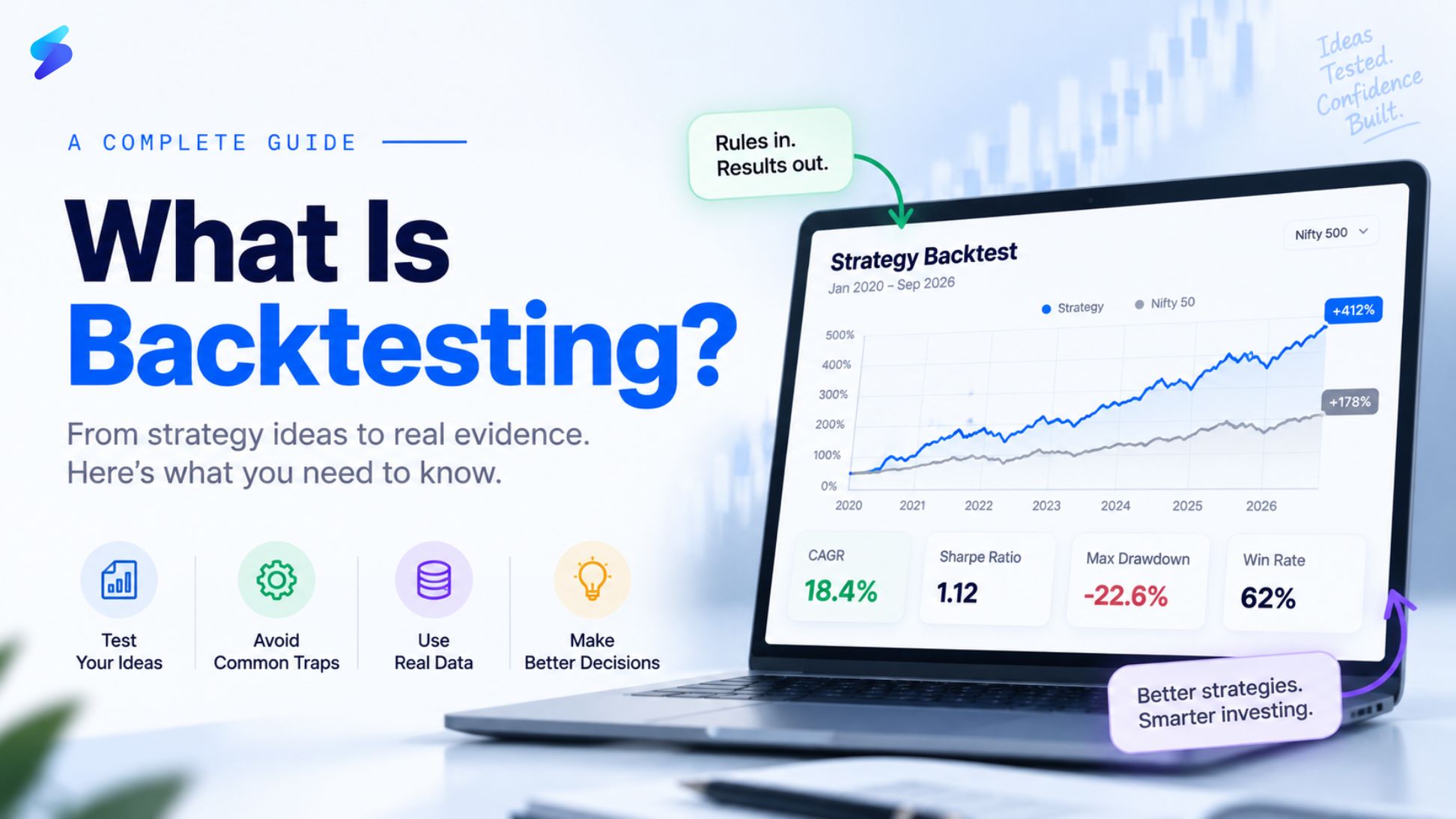
A backtest simulates a strategy by applying a defined set of rules to historical data and tracking the hypothetical portfolio that would have resulted. At its core, it answers one question: if I had followed these rules in the past, what would have happened?
A simple example: suppose your strategy is to buy the top 20 stocks ranked by 6-month price momentum from the Nifty 500 universe, hold them for one month, and then rebalance. A backtest would go back to, say, January 2020, identify which 20 stocks had the highest 6-month returns as of that date, simulate buying them in equal weights, hold for one month, sell, identify the new top 20 as of February 2020, buy again, and so on through September 2026. The result is a simulated portfolio with a complete return history.
That return history can then be compared to a benchmark, typically the Nifty 50 or Nifty 500, and analysed across dozens of metrics: total return, annualised CAGR, volatility, maximum drawdown, win rate, Sharpe Ratio, and more.
The purpose is not to prove the strategy worked in the past; that is easy to engineer with enough data manipulation. The purpose is to build a well-founded expectation of how the strategy will behave going forward, based on how it behaved across a range of historical market conditions.
Why Bias-Free, Point-in-Time Data Is Everything
The most important, and most commonly violated, principle in backtesting is the use of bias-free, point-in-time data. This is what separates a backtest that means something from one that produces an illusion of performance.
Survivorship Bias: The Most Common Trap
Survivorship bias occurs when a backtest uses only the companies that currently exist in a universe, ignoring the companies that existed historically but have since been delisted, merged, or gone bankrupt. It is one of the most pervasive problems in retail backtesting.
Consider the Nifty 500. The current Nifty 500 is a list of the 500 companies that are successful enough to be in the index today. But in 2015, the Nifty 500 contained many different companies — some of which have since been removed because they underperformed, became insolvent, or were acquired. A backtest that uses the current Nifty 500 constituents and goes back to 2015 is effectively selecting its investment universe from the future; it knows which companies survived, and naturally avoids the ones that did not.
The result is an artificially inflated return, because the backtest never holds any company that went to zero or was delisted at a loss. In reality, any investor running that strategy in 2015 would have owned some of those companies. The backtest does not reflect what they would have experienced.
A survivorship-bias-free backtest uses a complete historical universe that includes all companies that were in the investment universe at the time, including those that subsequently failed. This is what separates a meaningful backtest from a flattering one.
Look-Ahead Bias: Using Information That Did Not Exist Yet
Look-ahead bias occurs when a backtest uses data that would not have been available to an investor at the time the decision was being made. This is subtler than survivorship bias but equally damaging.
The most common example: financial data. A company’s Q1 FY26 results are filed with BSE in August 2026. If a backtest uses those results to make investment decisions for July 2026, before the results were filed, it has look-ahead bias. The strategy appears to know things that were not yet public information.
This is why point-in-time data is essential. Every data point used in a backtest must reflect what was actually available to an investor at the exact moment the simulated decision was made, not what was later reported, revised, or restated. Revenue figures get restated. EPS estimates get revised. Index constituents get updated retroactively. A backtest that does not handle these correctly produces results that are literally impossible to have achieved.
Overfitting: Designing Rules That Work in the Past But Not the Future
Overfitting is the subtlest and most intellectually dangerous of the biases. It happens when a strategy is designed, consciously or unconsciously, by tweaking parameters until the backtest looks good, rather than starting from a logical thesis and testing it.
With enough parameters and enough tweaking, you can always make a strategy look impressive on historical data. Change the momentum lookback from 6 months to 7 months. Adjust the P/E threshold from 25 to 22. Add a market cap filter. Each tweak improves the backtest slightly. By the time you have made twenty such adjustments, the strategy fits the historical data perfectly, and will almost certainly fail going forward, because you have optimised for noise rather than signal.
The antidote to overfitting is twofold. First, start from an economic or behavioural rationale, use factors and thresholds that have logical explanations for why they should work, not just ones that happened to work in your specific dataset. Second, test the strategy across multiple market regimes, bull markets, bear markets, sideways markets, high-volatility periods, and check that it holds up reasonably across all of them rather than working spectacularly in one specific period.
How to Read a Backtest Report: The Metrics That Matter
A well-constructed backtest generates dozens of metrics. Not all of them are equally important. Here is a structured guide to reading a backtest report — organised from the metrics that matter most to those that provide supporting context.
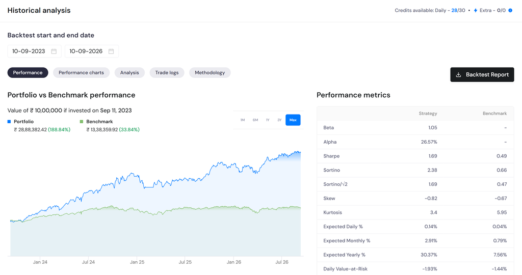
1. CAGR vs Benchmark CAGR: Does the Strategy Actually Outperform?
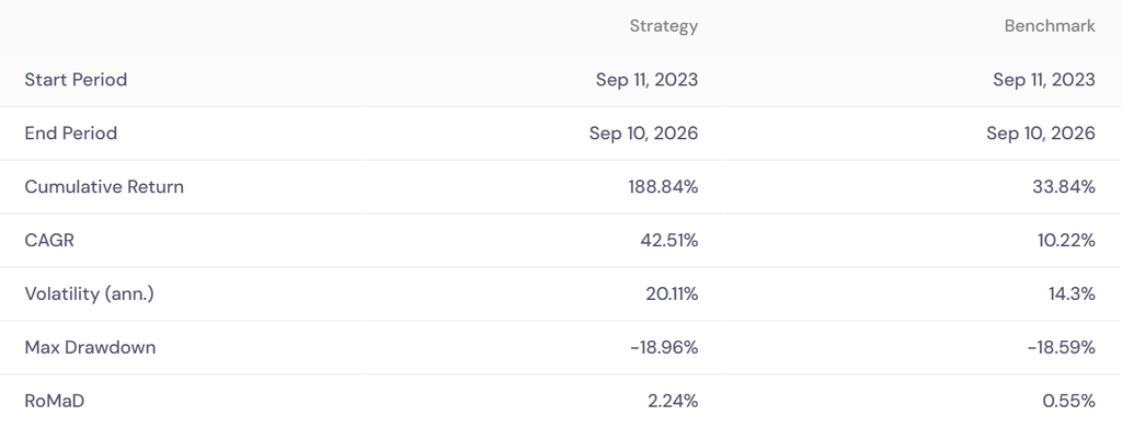
The first and most obvious question: does the strategy beat the benchmark? CAGR (Compound Annual Growth Rate) is the annualised return of the strategy over the backtest period. Comparing it to the benchmark CAGR tells you whether the strategy adds value above simply holding an index fund.
A strategy that delivers 18% CAGR against a benchmark CAGR of 13% has outperformed by 5 percentage points annually. Compounded over 5 years, that is the difference between a ₹10 lakh investment growing to ₹22.9 lakh (strategy) versus ₹18.5 lakh (benchmark).
However, CAGR alone is insufficient. A strategy with a higher CAGR that also has significantly higher volatility and deeper drawdowns may not be worth the additional risk — which is why the metrics below are necessary complements.
2. Cumulative Return: The Absolute Picture
Cumulative return shows the total gain from the start to the end of the backtest period, not annualised. It is the simplest expression of what happened to a notional investment. Seeing a portfolio grow from ₹10 lakh to ₹24 lakh (+141%) against a benchmark growth of 37% over the same period immediately communicates the magnitude of outperformance in terms any investor can understand.
3. Maximum Drawdown: The Worst You Would Have Experienced
Maximum drawdown (Max DD) measures the largest peak-to-trough decline in the portfolio’s value over the backtest period, the worst loss you would have experienced if you had invested at the worst possible time. This is the most important risk metric in a backtest.
A strategy with a Max DD of –35% is telling you: at some point in the backtest, if you had invested at the peak, you would have watched your portfolio lose 35% of its value before recovering. The question you must honestly answer is: could you have held through that? An investor who would have sold during a 35% drawdown — which most retail investors would — cannot practically use a strategy that requires holding through one.
Always compare the strategy’s Max DD to the benchmark’s Max DD. A strategy with a higher CAGR but also a significantly higher Max DD is taking on more risk to generate those returns. Whether that trade-off is acceptable depends entirely on your risk tolerance.
4. Sharpe Ratio: Return Per Unit of Risk
The Sharpe Ratio measures how much excess return the strategy generates for each unit of volatility it takes on. A higher Sharpe Ratio means more return per unit of risk, a more efficient strategy. The formula is: (Strategy Return – Risk-Free Rate) ÷ Standard Deviation of Returns.
As a rough guide: a Sharpe Ratio above 1.0 is generally considered good for an equity strategy; above 1.5 is strong. A strategy with a Sharpe of 1.3 vs a benchmark Sharpe of 0.5 is delivering significantly better risk-adjusted returns — not just higher raw returns, but higher returns relative to the volatility the investor has to absorb.
5. Sortino Ratio: Penalising Only Downside Volatility
The Sortino Ratio is a refinement of the Sharpe Ratio. Where Sharpe penalises all volatility — both upside and downside — the Sortino Ratio only penalises downside volatility (returns below the minimum acceptable return). This is arguably more meaningful for investors who do not mind volatile upside but want to minimise volatile downside.
A strategy with a high Sortino Ratio relative to both its Sharpe and the benchmark’s Sortino indicates that most of its volatility is on the upside — the kind of volatility investors actually welcome.
6. Alpha: What the Strategy Added Beyond Market Exposure
Alpha measures the return generated by the strategy above and beyond what its market exposure would predict. A Beta of 1.03 and an Alpha of 20% means the strategy moved broadly in line with the market (beta close to 1) but generated 20 percentage points of additional annual return that cannot be explained by simply riding market direction. That additional return is the strategy’s value-add, its excess performance attributable to stock selection or timing rather than market exposure.
7. RoMaD: Return Over Maximum Drawdown
RoMaD (Return over Maximum Drawdown) is a practical risk-adjusted metric that divides the strategy’s annualised return by its maximum drawdown. It answers: for every rupee of maximum loss I would have had to absorb, how much annual return did I get?
A RoMaD of 1.4 means the strategy generated 1.4x its maximum drawdown in annual returns, a reasonable trade-off. The benchmark’s RoMaD is the comparison point. If the strategy’s RoMaD is significantly higher than the benchmark’s, the strategy is generating more return per unit of maximum downside risk — a strong signal of quality beyond raw performance.
8. Calendar Year Returns: Does It Hold Up Across Different Markets?
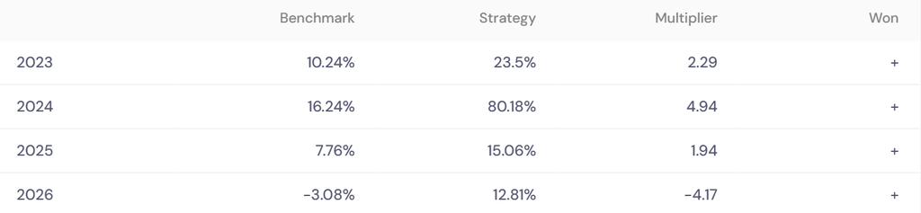
Calendar year returns break the backtest into annual slices and compare the strategy against the benchmark year by year. This is one of the most revealing sections of any backtest report because it shows whether the outperformance is consistent or concentrated in one or two lucky years
A strategy that outperformed in 2023 (+14% vs +12%), 2024 (+31% vs +16%), 2025 (+30% vs +8%), and 2026 YTD (+24% vs –2%) is demonstrating consistent outperformance across multiple different market environments — a bull year, a volatile year, and a down year. That consistency is far more meaningful than a single year of spectacular outperformance with mediocre performance in all others.
Pay particular attention to down-market years, years where the benchmark was negative or flat. A good strategy should ideally show smaller losses than the benchmark in bad years (capital protection) while delivering larger gains in good years (upside participation). If the strategy only outperforms in strong bull markets but underperforms badly when markets fall, it is a leveraged market bet rather than a genuine alpha-generating strategy.
9. Trade Summary Metrics: The Mechanical Reality
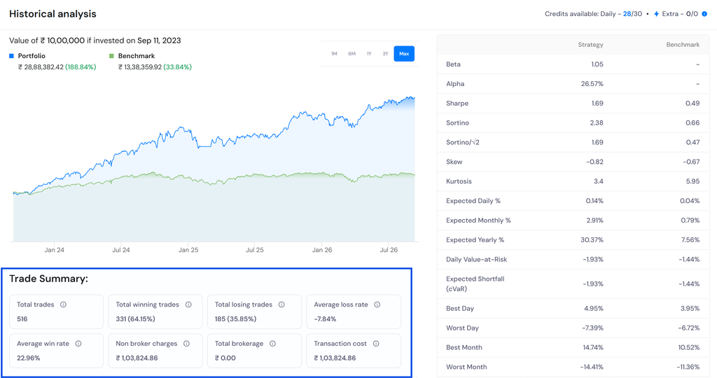
The trade summary shows the mechanics of how the strategy generates returns. Key metrics:
Win Rate: What percentage of individual trades were profitable. A win rate of 60% means 6 out of every 10 trades made money. Note that win rate alone is meaningless without knowing the average win and average loss sizes; a strategy with a 40% win rate but an average win 3x larger than the average loss is profitable overall.
Average Win vs Average Loss: The relationship between these two numbers is the strategy’s profit factor, the ratio of average gain to average loss. A strategy with an average win of 18% and an average loss of 4.5% has a profit factor of 4:1, meaning even with a win rate below 50%, the strategy is significantly profitable because winners are much larger than losers.
Total Trades: A low number of trades can make statistical significance questionable. A strategy that made 15 trades over 3 years may look impressive but does not have enough data points to draw reliable conclusions. A strategy with 500+ trades provides much stronger statistical evidence that the results are not due to chance.
10. Trailing Returns: How It Looks Across Different Time Windows
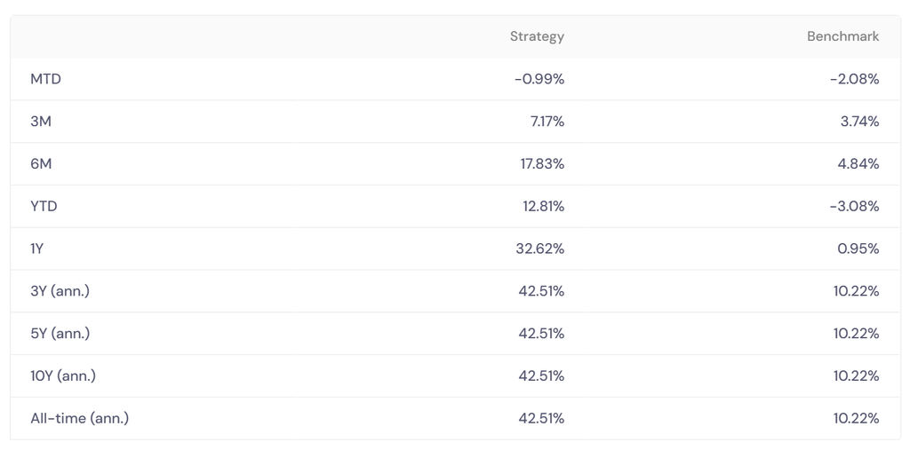
Trailing returns show performance across multiple fixed windows ending on the backtest’s end date: month-to-date, 3 months, 6 months, 1 year, 3 years, 5 years. This is useful for understanding how the strategy has performed in recent periods relative to its longer-term average.
A strategy showing strong 1-year trailing returns that are significantly above its 3-year annualised CAGR is in a period of unusual outperformance, which may mean the strategy is overheated and due to revert, or it may reflect genuine acceleration. A strategy where recent trailing returns are below the long-term CAGR is in a period of relative underperformance, which may or may not be a concern depending on whether there is a logical reason for the weakness.
Advanced Risk Metrics: What the Numbers Below the Headline Tell You
| Metric | What It Measures | What to Look For |
| Volatility (ann.) | Standard deviation of returns, annualised | Lower is better for the same return. Compare to benchmark; significant excess volatility requires a commensurate return premium. |
| Daily VaR (Value at Risk) | Maximum expected daily loss at a 95% confidence level | A VaR of –2% means you should not expect to lose more than 2% on any given day more than 5% of the time. Higher VaR = higher tail risk. |
| Expected Shortfall (cVaR) | Average loss on the days when VaR is breached | More conservative than VaR, captures the severity of tail events, not just the probability of them. Important for understanding worst-case scenarios. |
| Longest Drawdown Days | How many consecutive days the portfolio was below its previous peak | A long drawdown duration tests investor patience. A strategy that takes 2 years to recover from a drawdown will see many investors abandon it before the recovery. |
| Win Quarter % / Win Year % | Percentage of quarters or years where strategy beat benchmark | High win-quarter and win-year percentages indicate consistent rather than lumpy outperformance. 75%+ win year is a strong signal. |
| Best/Worst Month | The single best and single worst calendar month in the backtest | Shows the range of outcomes you might experience in any given month. Relevant for investors with shorter time horizons. |
| Skew | Asymmetry of the return distribution | Negative skew means the strategy occasionally has large losses (even if average performance is good). Positive skew is generally preferable — small frequent losses, occasional large gains. |
What Makes a Backtest Trustworthy: A Checklist
Before trusting any backtest result, including your own, run through these questions:
1. Is the universe survivorship-bias free? Does the backtest include companies that were in the universe at the time, including those that were subsequently delisted or went bankrupt? If the universe is only current constituents projected back in time, the results are inflated.
2. Is point-in-time data used? Are financial metrics calculated using only data that was publicly available at the time each decision was made? If quarterly results filed in August are being used for July decisions, there is look-ahead bias.
3. Does the strategy have an economic or behavioural rationale? Is there a logical reason why the strategy should work — a factor premium, a behavioural bias being exploited, an information edge? Or does the strategy appear to work only because it was tuned to fit the historical data?
4. Has it been tested across multiple market regimes? Does the strategy hold up in bull markets and bear markets? In high-volatility and low-volatility environments? In large-cap-dominated periods and small-cap periods? A strategy that only works in one type of market is not a robust strategy.
5. Are transaction costs included? Brokerage, STT, exchange charges, and bid-ask spreads are real costs that compound over hundreds of trades. A strategy that generates 20% annual returns before costs but makes 200 trades per year with significant transaction costs per trade may net much less. Costs must be modelled realistically.
6. Is the backtest period long enough? A 2-year backtest that happened to be a strong bull market proves very little. A good backtest covers at least one full market cycle, including a significant correction, to show how the strategy behaves across different conditions. Five to seven years is the minimum; ten years or more is meaningfully better.
7. How many rules and parameters does the strategy have? Simpler strategies with fewer parameters are less likely to be overfit. A 20-condition strategy that produces excellent backtested results is far more suspicious than a 4-condition strategy with similar results — because the more conditions, the more opportunities to have tuned them to historical data.
Running a Backtest on sharpely
sharpely’s Strategy Builder includes a built-in backtest engine designed around the principles described above. The backtest uses survivorship-bias-free historical data, meaning the universe at each rebalancing date reflects the companies that actually existed and were tradeable at that time, not the current universe projected backwards. Financial data used for screening is point-in-time; the screener conditions at each rebalancing date use only data that was publicly available as of that date.
When you build a strategy on sharpely, defining entry conditions, exit conditions, stop-loss rules, position sizing, and rebalancing frequency, the backtest simulates every rebalancing decision across the historical period you select. The output includes the full suite of metrics discussed in this article: portfolio growth vs benchmark, CAGR, Max Drawdown, Sharpe, Sortino, Alpha, RoMaD, calendar year returns, trailing returns, trade summary statistics, and the full range of risk metrics including VaR, Expected Shortfall, and drawdown analysis.
Transaction costs: STT, exchange charges, and other non-broker costs are modelled and shown separately, so you can see the net performance after realistic costs rather than a pre-cost figure that overstates what you would actually have earned.
The backtest report also includes trade logs, a record of every simulated buy and sell decision, which stock was traded, at what price, and what the outcome was. This lets you audit the strategy’s historical decisions rather than just accepting the aggregate statistics.
Key Takeaways
Backtesting is the closest thing to a scientific experiment for investment strategies. It applies defined rules to historical data and shows what would have happened, turning a hypothesis into evidence.
The data quality is more important than the results. A backtest built on survivorship-biased or non-point-in-time data produces results that are literally impossible to have achieved. Bias-free, point-in-time data is the non-negotiable foundation of any valid backtest.
CAGR is the headline; Max Drawdown is the truth. High CAGR with a drawdown you could not have psychologically held through is a strategy you cannot practically use. Always read both together.
Sharpe, Sortino, and RoMaD reveal whether the returns are efficient. A strategy that generates 20% CAGR with a Sharpe of 0.4 is taking on enormous risk for that return. One with 18% CAGR and a Sharpe of 1.4 is doing the same job far more efficiently.
Calendar year returns and trade statistics reveal whether results are consistent or lucky. Consistent outperformance across multiple different market environments, including a down year, is the strongest signal that a strategy has a genuine edge rather than good timing.
A great backtest is the beginning of the process, not the end. A strategy that passes all the checks above is worth deploying carefully, with small initial capital, monitored closely, and adjusted if its real-world performance diverges systematically from its backtest behaviour in ways that cannot be explained by market regime differences.